Example Figures

To make your figures accessible to as many readers as possible, try to avoid conveying information using only colour differences. In graphs and plots use symbols, labels, line styles or fill patterns to indicate different data, in addition to different colours.

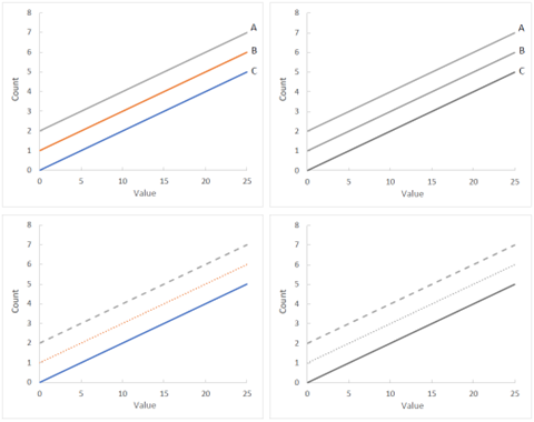
Figure 1. Demonstration of using labels or line styles so that information is clear when figures are converted to greyscale. Left panels show lines in different colours which are very similar when converted to greyscale (right panels). The lines are easy to distinguish by using either labels (top panels) or line styles (bottom panels). The same principle can be applied to other types of chart.

It is not always possible to have good colour contrast or to use labels or symbols, for example with photographic images or colour gradient maps.

For all figures it is important to use the figure caption to provide a description of the information that the figure conveys so that all readers, including those using screen-reader technology, can understand why the image is present. Figure captions must be understandable without needing to refer to the main text of the article.

Figures 2-5 are examples taken from published articles to demonstrate use of the figure caption to describe the information that the image conveys.

 

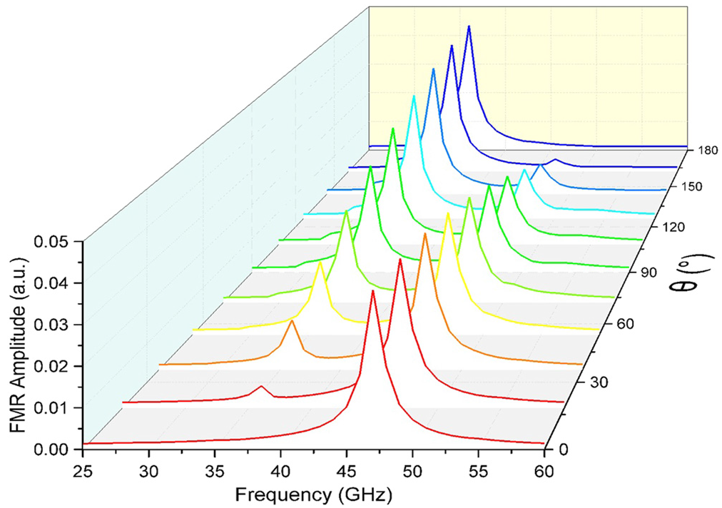
Figure 2. FMR response curves of PMA–SAF as a function of the phase factor θ of microwave fields. Here H₀ = 2 kOe, h₀ = 30 Oe and θ varies from 0° to 180°. The resonance signal amplitude of the LH mode increases while that of RH mode decreases with θ increasing. [Example figure taken from Chen X et al 2021 New J. Phys. 23 113029 https://iopscience.iop.org/article/10.1088/1367-2630/ac3556]

 

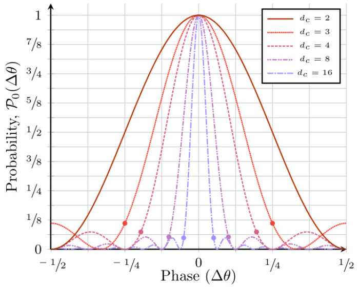
Figure 3. Plot of 𝒫₀(Δθ) (equation (3)) from Δθ ∈ [−.5, .5) for various d_c . Note that 𝒫₀ has infinite domain with period 1. Probability of the (d_c -level) control register of an IPEA collapsing to |0⟩ as a function of difference between the eigenphase θ and the applied rotation θ_R , Δθ ≡ θ − θ_R for an eigenstate input. Note that when the applied rotation matches the eigenphase (Δθ = 0), the control collapses to |0⟩ deterministically. Denote the region around Δθ = 0 (from dot to dot) as the central lobe of 𝒫₀(Δθ), and the small lobes with local maxima outside of it as the sidelobes. See that the higher the system’s dimensionality, the narrower the probability curve’s central lobe and the lower local maxima in the sidelobes. Note that d_c = 2 has no sidelobes (the probability is monotonic on either side of the central lobe). Also note 𝒫₀(Δθ) = 0 for Δθ = d_c^-1 and the width of the central lobe is therefore Δθ_FWHM = 2 d_c^-1. [Example figure taken from Moore A J et al 2021 New J. Phys. 23 113027 https://iopscience.iop.org/article/10.1088/1367-2630/ac320d]

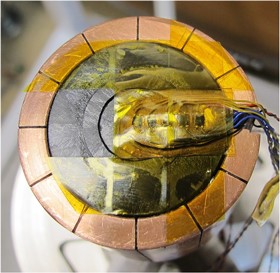
Figure 4. Sample assembly arrangement. Three Hall sensors are positioned on the inner core, and two sensors are on the ring. The distance between adjacent sensors is 2.5 mm. A further sensor is placed inside the bore of the ring. [Example figure taken from Zhou D et al 2020 Supercond. Sci. Technol. 33 034001 https://iopscience.iop.org/article/10.1088/1361-6668/ab66e7]

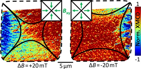
Figure 5. Local XMCD pattern inside the YBCO(250 nm)/Py(50 nm) bilayer at T = 26 K after zero field cooling. The positions of the flux fronts/d-lines are marked by black lines. (Left) Increasing the external magnetic field from −40 to −20 mT (ΔB = +20 mT) leads to supercurrents flowing clockwise inside the sample. Here, the local magnetic field points towards the center of the square enhancing the penetration of magnetic flux (black lines). (Right) In case of ΔB = −20 mT (+40 to +20 mT) supercurrents flow anti-clockwise, reversing the latter effect. [Example figure taken from Simmendinger J et al 2020 Supercond. Sci. Technol. 33 025015 https://iopscience.iop.org/article/10.1088/1361-6668/ab54ab]